Improving Imbalanced Machine Learning with Neighborhood-Informed Synthetic Sample Placement

Figures supplement

Figure 1. Calculation of the sum of the distances between a minority sample and its k-nearest minority neighbors (k=3)

Figure 2. Demonstration of the loneliness function

Figure 3. Finding local variation

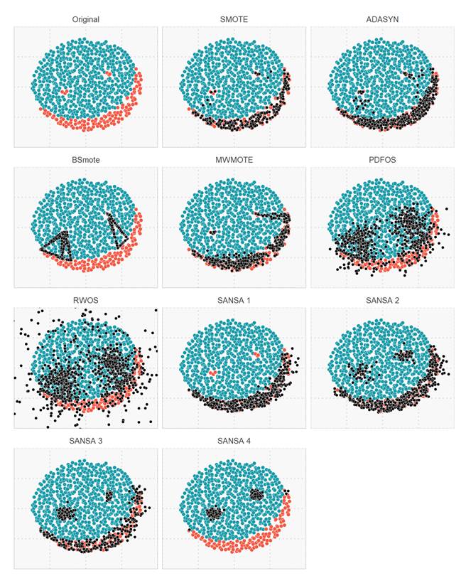
Figure 4. Example of synthetic sample generation on a hypothetical 3-dimensional dataset

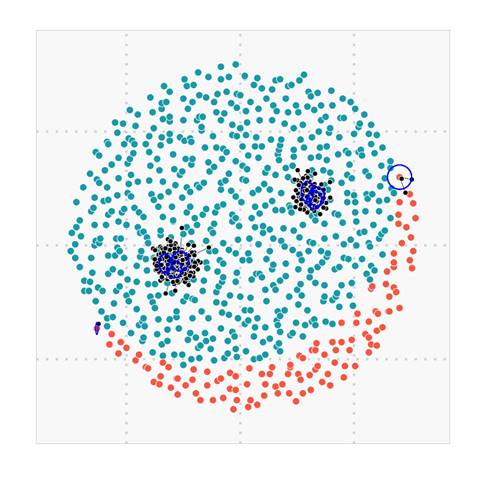
Figure 5. (a) Large  leads to most synthetic points generated around loneliest minority points

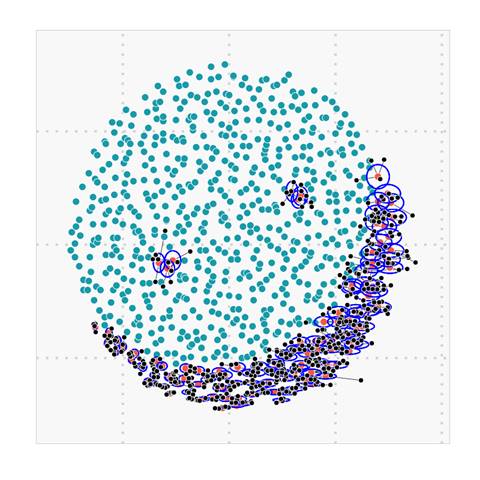
Figure 5. (b)  leads to synthetic points equally distributed for all existing minority points

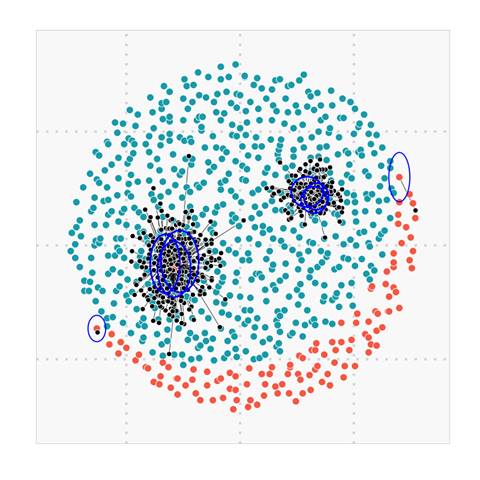
Figure 5. (c) Larger k results in larger spread for synthetic points around their respective originating minority points

Figure 5. (d) Changing k

Figure 5. (e) Changing Lambda

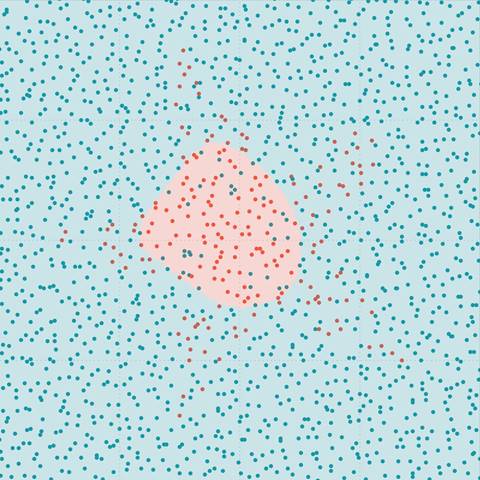
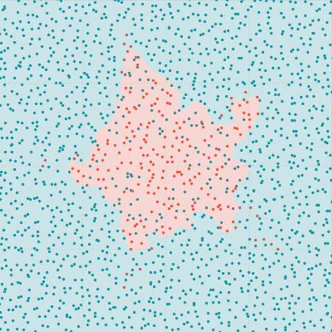
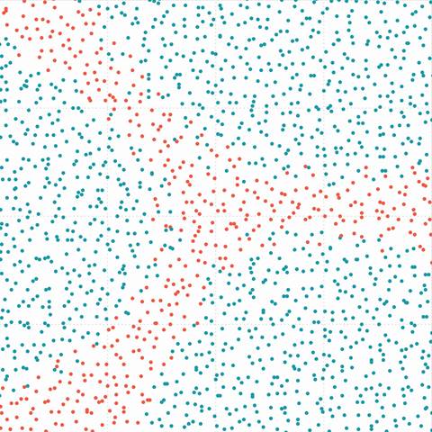
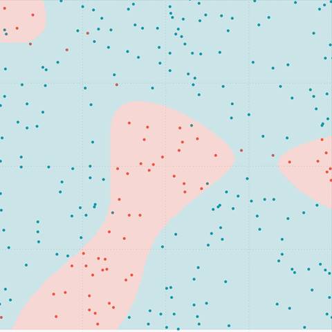
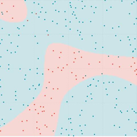
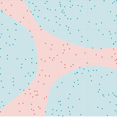
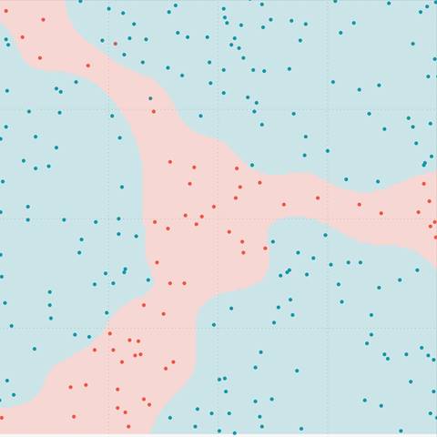
Figure 6. (a) Original data (left) with prediction map (right)

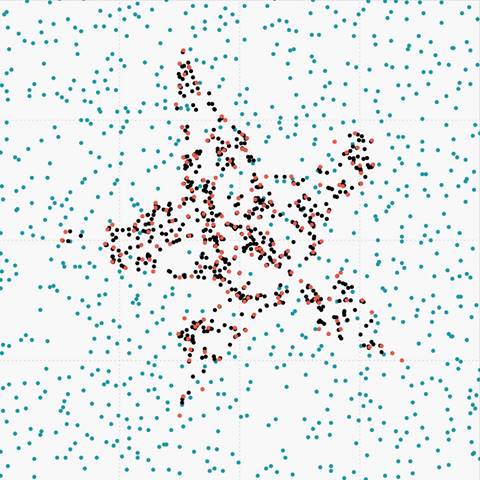
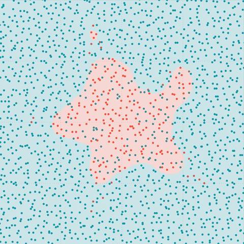
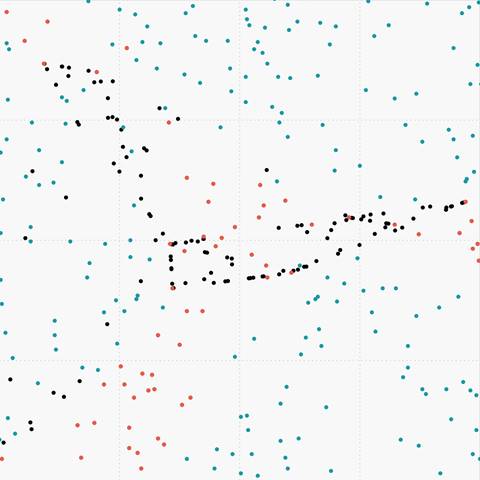
Figure 6. (b) Overlapped data

Figure 6. (c) Overlapped data oversampled with SMOTE

Figure 6. (d) Overlapped data oversampled with MWMOTE

Figure 6. (e) Overlapped data oversampled with ADASYN

Figure 6. (f) Overlapped data oversampled with BSMOTE

Figure 6. (g) Overlapped data oversampled with PDFOS

Figure 6. (h) Overlapped data oversampled with RWOS

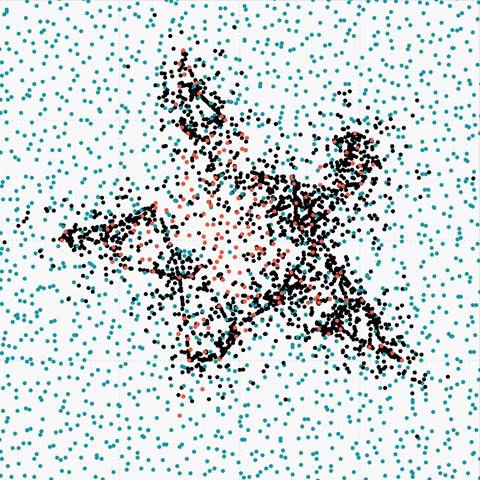
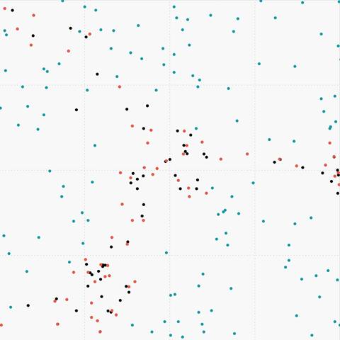
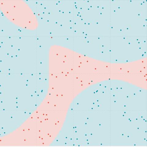
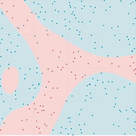
Figure 6. (i) Overlapped data oversampled with SANSA

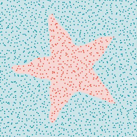
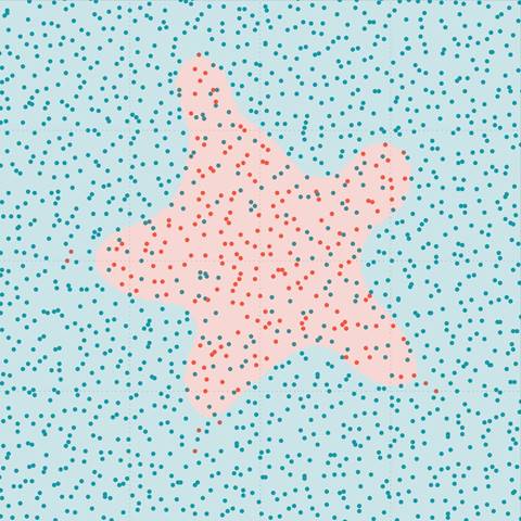
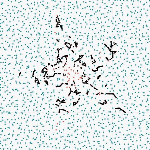
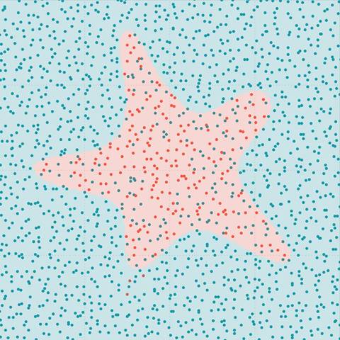
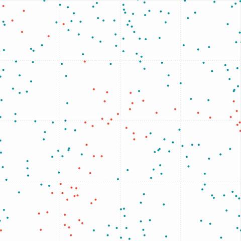
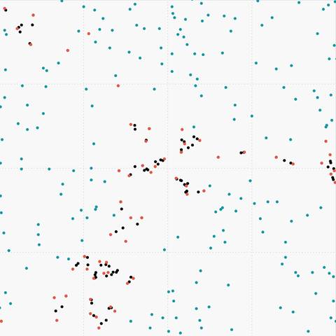
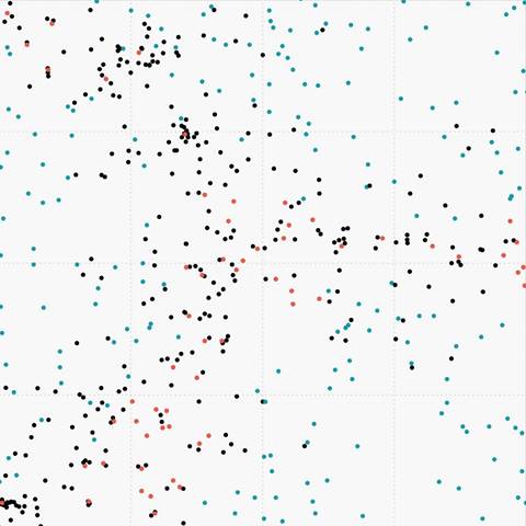
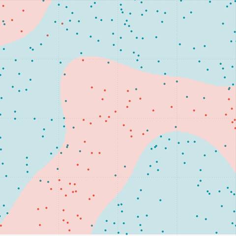
Figure 7. (a) Original data (left) with prediction map (right)

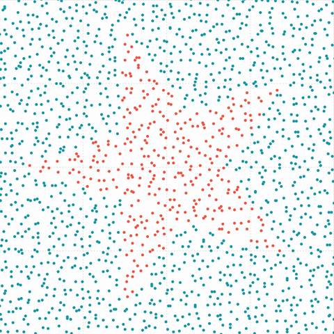
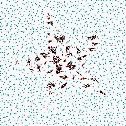
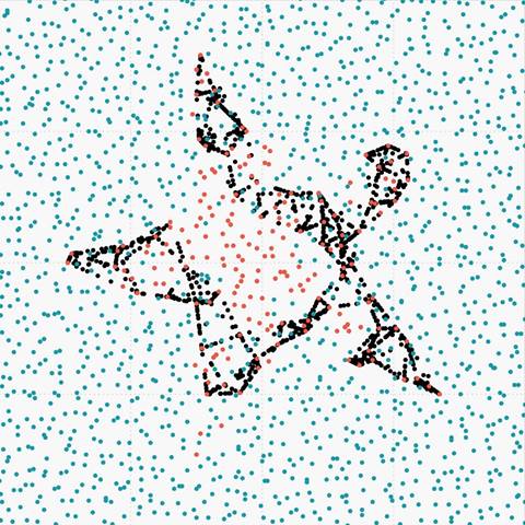
Figure 7. (b) Sparse data

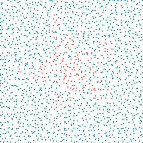
Figure 7. (c) Sparse data oversampled with SMOTE

Figure 7. (d) Sparse data oversampled with MWMOTE

Figure 7. (e) Sparse data oversampled with ADASYN

Figure 7. (f) Sparse data oversampled with BSMOTE

Figure 7. (g) Sparse data oversampled with PDFOS

Figure 7. (h) Sparse data oversampled with RWOS

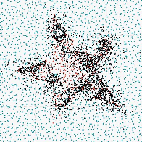
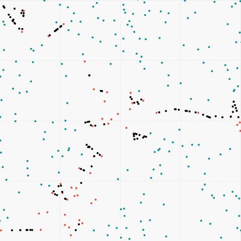
Figure 7. (i) Sparse data oversampled with SANSA

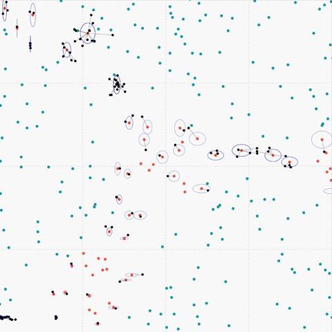
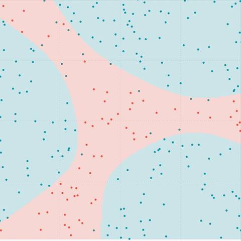
Figure 8. Imbalanced Learning Framework using SANSA